Bike Sharing Demand in Washington with Random Forest

In this predictive modeling project, our focus is on forecasting bike rental demand within the Capital Bikeshare program in Washington, D.C. The dataset at our disposal comprises historical information, including weather data, obtained from the Bike Sharing Demand dataset on Kaggle. To tackle this regression problem and predict the number of bike rentals, we have chosen to employ the Random Forests algorithm. Random Forests, being an ensemble learning method, harnesses the power of multiple decision trees to collectively provide accurate and robust predictions. By leveraging features such as temperature, humidity, and wind speed from the historical data, the Random Forests algorithm will learn complex patterns and relationships to make predictions about the bike rental demand. This project not only demonstrates the application of machine learning in predicting real-world scenarios but also highlights the versatility of Random Forests in handling complex, multi-dimensional datasets for demand forecasting.

import pandas as pd

import matplotlib.pyplot as plt
import seaborn as sns

from sklearn.ensemble import RandomForestRegressor
from sklearn.ensemble import GradientBoostingRegressor

from sklearn.model_selection import train_test_split
from sklearn.model_selection import GridSearchCV

from sklearn.metrics import mean_squared_error as MSE

df_bikes = pd.read_csv('bikes.csv')
print(df_bikes)

sns.set_palette("rocket")

Data Visualization

# Create a jointplot similar to the JointGrid
sns.jointplot(x="hum",
        y="cnt",
        kind='reg',
        data=df_bikes)

plt.show()
plt.clf()

# Plot temp vs. total_rentals as a regression plot
sns.jointplot(x="temp",
         y="cnt",
         kind='reg',
         data=df_bikes,
         order=2,
         xlim=(0, 1)
         )

plt.show()
plt.clf()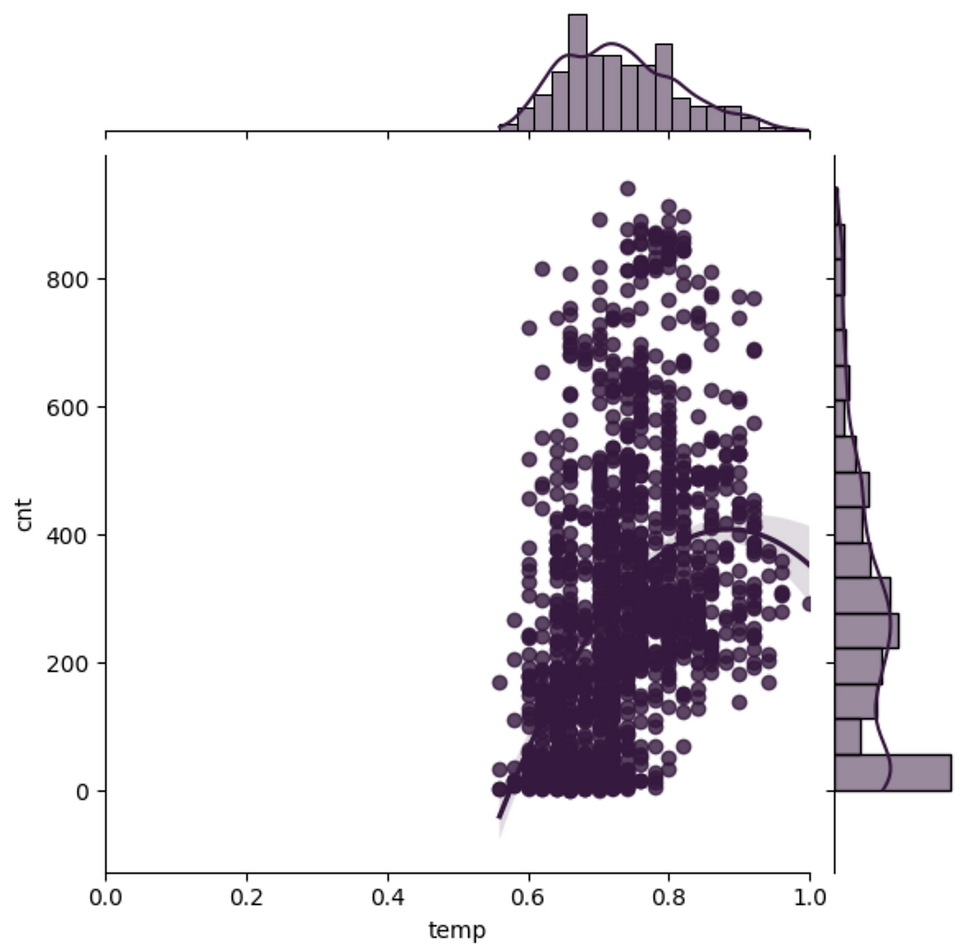

# Replicate the above plot but only for registered riders
g = sns.jointplot(x="windspeed",
             y="cnt",
             kind='scatter',
             data=df_bikes,
             marginal_kws=dict(bins=10))
g.plot_joint(sns.kdeplot)

plt.show()
plt.clf()

Train/Test split

X = df_bikes.drop(['cnt'], axis=1)
y = df_bikes[['cnt']]

X_train, X_test, y_train, y_test = train_test_split(X, y, test_size=0.2, random_state=4)

RandomForest Model

# Instantiate rf
rf = RandomForestRegressor(n_estimators=25, random_state=2)

# Fit to the training data
rf.fit(X_train, y_train)

Evaluate RF

# Predict on test data
y_pred = rf.predict(X_test)

# Evaluate the test
rmse_test = MSE(y_test, y_pred) ** (1/2)

print('Test set RMSE of rf: {:.3f}'.format(rmse_test))

Test set RMSE of rf: 50.424 The test set RMSE achieved by rf is significantly smaller than that achieved by a single CART!

Feature importance

# Create a pd.Series of features importance
importances = pd.Series(data=rf.feature_importances_, index=X_train.columns)

# sort importances
importances_sorted = importances.sort_values()

# Barplot
importances_sorted.plot(kind='barh', color='lightgreen')
plt.title('Feature Importances')
plt.show()

Gradient Boosting regressor

# Instantiate GB
gb = GradientBoostingRegressor(max_depth=4, n_estimators=200, random_state=2)

# Fit
gb.fit(X_train, y_train)

# Predict
y_pred = gb.predict(X_test)

Evaluate GB

# MSE
mse_test = MSE(y_test, y_pred)

# RMSE
rmse_test = mse_test ** (1/2)

print('Test set RMSE of gb: {:.3f}'.format(rmse_test))

Test set RMSE of gb: 50.340

Stochastic Gradient Boosting Regressor

# Instantiate sgbr
sgbr = GradientBoostingRegressor(max_depth=4,
            subsample=0.9,
            max_features=0.75,
            n_estimators=200,
            random_state=2)

# Fit sgbr to the training set
sgbr.fit(X_train, y_train)

# Predict test set labels
y_pred = sgbr.predict(X_test)

Evaluate SGBR

# Compute test set MSE
mse_test = MSE(y_test, y_pred)

# Compute test set RMSE
rmse_test = mse_test ** (0.5)

# Print rmse_test
print('Test set RMSE of sgbr: {:.3f}'.format(rmse_test))

Test set RMSE of sgbr: 50.294

Hyperparameter grid of RF

# Define the dictionary 'params_rf'
params_rf = {"n_estimators":[100, 350, 500], 'max_features': ['log2', 'auto', 'sqrt'], 'min_samples_leaf': [2, 10, 30]}

# Instantiate grid_rf
grid_rf = GridSearchCV(estimator=rf, param_grid=params_rf, scoring='neg_mean_squared_error', cv=3, verbose=1, n_jobs=-1)

grid_rf.fit(X_train, y_train)

Evaluate optimal forest

 Best estimator
best_model = grid_rf.best_estimator_

# Predict
y_pred = best_model.predict(X_test)

# Compute rmse_test
rmse_test = MSE(y_test, y_pred) ** (1/2)

# Print rmse_test
print('Test RMSE of best model: {:.3f}'.format(rmse_test))

Test RMSE of best model: 47.950

Reference:

https://www.datacamp.com/