Electricity Consumption Time Series Data visualization

Embarking on an in-depth exploration of time-series data within the Building Data Genome Project, our focus centers on unraveling the intricacies of electricity energy consumption in the context of office buildings. Adopting a comprehensive approach, we intend to analyze the temporal patterns of energy usage and correlate them with pertinent weather data to discern the impact of climatic conditions on energy demands. By specifically honing in on office spaces, we aim to uncover nuanced insights into how weather variations influence the electricity consumption dynamics within professional environments. This multifaceted investigation not only illuminates the unique energy profiles of office buildings but also seeks to establish connections between external meteorological factors and the fluctuating energy needs of these spaces. Through this integrated analysis, we aspire to contribute valuable knowledge that aids in optimizing energy efficiency strategies tailored specifically for office infrastructures within the Building Data Genome Project.

import pandas as pd

directory = 'meter_data/'

abigail = pd.read_csv(directory + 'Office_Abigail.csv', index_col = "timestamp", parse_dates=True) 

abigail.info()

abigail.index[0]

Timestamp('2015-01-01 00:00:00')

abigail.index

Plotting Time-Series Charts

abigail.plot()

abigail.plot(marker='.', alpha=0.5, linestyle='None', figsize=(15, 5))

Resample the data to other frequencies

abigail_daily = abigail.resample("D").mean()

abigail_daily.plot(figsize=(10,5))

abigail_daily.resample("M").mean().plot(figsize=(10,5))

abigail_daily_june = abigail_daily.truncate(before = '2015-06-01', after='2015-07-01')

abigail_daily_june.plot(figsize=(10,5))

Trends Analysis and Rolling Windows

abigail.rolling(window=500, center=True, min_periods=500).mean().plot()

list_of_buildings = ['UnivClass_Andy.csv',
'Office_Abbey.csv',
'Office_Alannah.csv',
'PrimClass_Angel.csv',
'Office_Penny.csv',
'Office_Pam.csv',
'UnivClass_Craig.csv',
'UnivLab_Allison.csv',
'Office_Amelia.csv',
'Office_Aubrey.csv']

all_data_list = []
for buildingname in list_of_buildings:
  df = pd.read_csv(directory + buildingname, index_col = "timestamp", parse_dates=True) 
  df = df.resample("H").mean()
  all_data_list.append(df)
all_data = pd.concat(all_data_list, axis=1)

all_data.info()

all_data.plot(figsize=(20,30), subplots=True);

all_data.resample("D").mean().plot(figsize=(20,30), subplots=True);

all_data.resample("D").mean().truncate(after='2015-06-01').plot(figsize=(20,30), subplots=True)

Normalization based on floor area

meta = pd.read_csv("all_buildings_meta_data.csv", index_col="uid")

meta.loc[buildingname]

rawdata_normalized = rawdata/meta.loc[buildingname]["sqm"]

rawdata_normalized_monthly = rawdata_normalized.resample("M").sum()

rawdata_normalized_monthly.plot(kind="bar", figsize=(10,4), title='Energy Consumption per Square Meter Floor Area')

Automation of the process of analysis on multiple buildings

buildingnamelist = ["Office_Abbey",
"Office_Pam",
"Office_Penny",
"UnivLab_Allison",
"UnivLab_Audra",
"UnivLab_Ciel"]

annual_data_list = []
annual_data_list_normalized = []

for buildingname in buildingnamelist:
    print("Getting data from: "+buildingname)
    
    rawdata = pd.read_csv(directory + buildingname + ".csv", parse_dates=True, index_col='timestamp')
    floor_area = meta.loc[buildingname]["sqm"]
    
    annual = rawdata.sum()

    normalized_data = rawdata/floor_area
    annual_normalized = normalized_data.sum()
    
    annual_data_list_normalized.append(annual_normalized)
    annual_data_list.append(annual) 

totaldata = pd.concat(annual_data_list)
totaldata_normalized = pd.concat(annual_data_list_normalized)

Unnormalized energy consumption

totaldata.plot(kind='bar',figsize=(10,5))

Normalized Energy Consumption

totaldata_normalized.plot(kind='bar',figsize=(10,5))

Weather Influence

file = "UnivClass_Ciara.csv"
directory = 'meter_data/'

rawdata = pd.read_csv(directory + file, parse_dates=True, index_col='timestamp')

rawdata.info()

rawdata.plot(figsize=(10,4))

Load Weather Data

directory = 'weather_data/'
weather_data = pd.read_csv(directory + "weather2.csv", index_col='timestamp', parse_dates=True)

weather_data.info()

weather_data["TemperatureC"].plot(figsize=(10,4))

Finding and removing outliers

weather_hourly = weather_data.resample("H").mean()

weather_hourly_nooutlier = weather_hourly[weather_hourly > -40]

weather_hourly_nooutlier["TemperatureC"].plot(figsize=(10,4))

Filling gaps in data

weather_hourly_nooutlier_nogaps = weather_hourly_nooutlier.fillna(method='ffill')

Merge Temperature and Electricity Data - Combining Data Sets

comparison = pd.concat([weather_hourly_nooutlier_nogaps['TemperatureC'], rawdata['UnivClass_Ciara']], axis=1)

comparison.plot(figsize=(20,10), subplots=True)

Analyze the weather influence on energy consumption

comparison.plot(kind='scatter', x='TemperatureC', y='UnivClass_Ciara', figsize=(10,10))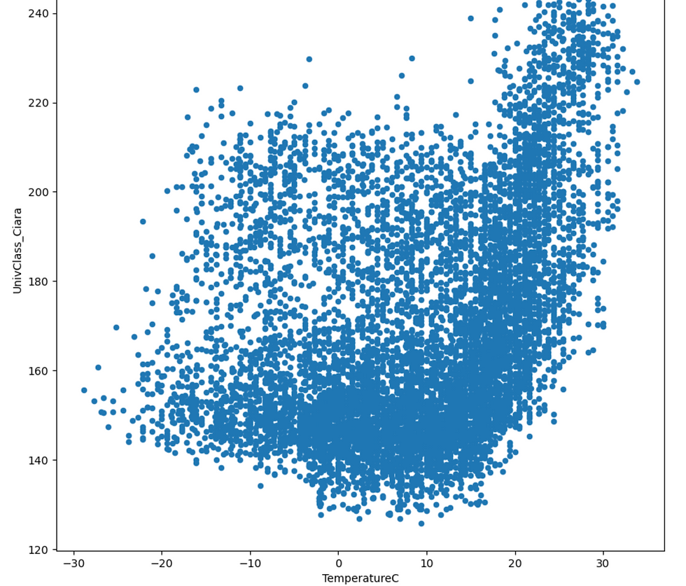

import seaborn as sns

def make_color_division(x):
  if x < 14:
    return "Heating"
  else:
    return "Cooling"

comparison = comparison.resample("D").mean()

comparison['heating_vs_cooling'] = comparison.TemperatureC.apply(lambda x: make_color_division(x))

g = sns.lmplot(x="TemperatureC", y="UnivClass_Ciara", hue="heating_vs_cooling",
               truncate=True, data=comparison)

g.set_axis_labels("Outdoor Air Temperature", "Average Hourly kWH")

Reference:

- Data Science for Construction, Architecture and Engineering by Clayton Miller (clayton@nus.edu.sg - miller.clayton@gmail.com): https://www.edx.org/learn/data-science/the-national-university-of-singapore-data-science-for-construction-architecture-and-engineering - Simulation files by Miguel Martin (miguel.martin@u.nus.edu.sg) - Building Data Genome Project: https://github.com/buds-lab/the-building-data-genome-project